How histogram is calculated in Prometheus
What is P99?#
P99 (or “99th percentile”) is a performance metric commonly used to describe latency or response-time behavior in systems.
P99 latency is the value under which 99% of all requests complete. That means only 1% of requests are slower than this threshold.
If your P99 is 200 ms, then 99 out of 100 requests were served in 200 ms or less; only 1 request was slower.
It highlights the “tail latency” — those rare, slow requests that the average hides but which can badly impact user experience.
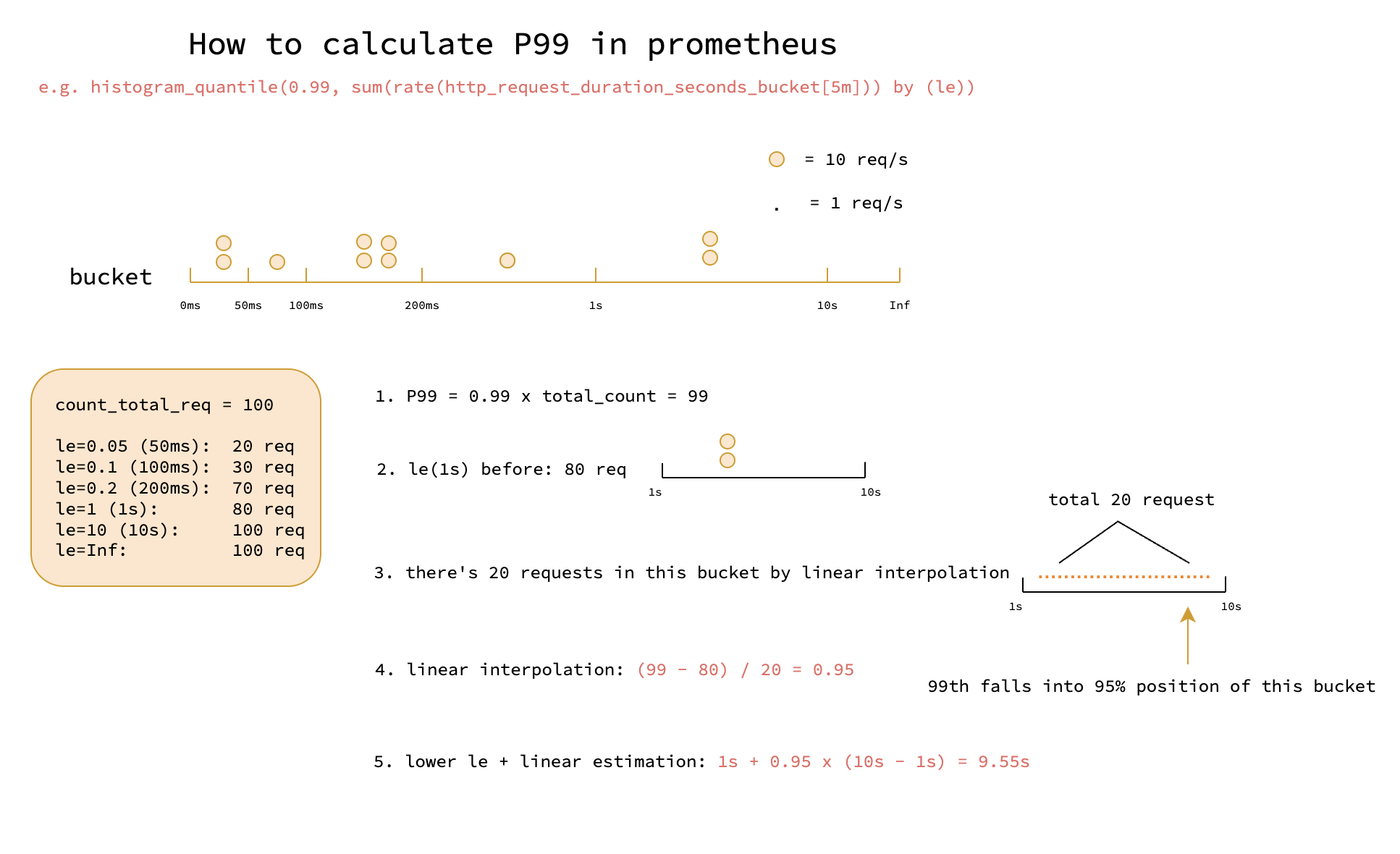
Diagram#
Calculation#
Before diving into the calculation of histogram, what’s histogram metric type? see details in Metric Type
Let’s start with a commmon histogram scenario: we want to calculate the p99 of the http request latency, the promql query is like this:
histogram_quantile(0.99, sum(rate(http_request_duration_seconds_bucket[5m])) by (le))
Let’s highlight 3 key points of histogram:
- histogram quantiles are estimated with linear interpolation, which means the result is not exact, but an estimation.
- histogram buckets are cumulative, for example, if we have http request duration buckets
[0.05, 0.1, 0.2, 1, 10], it means:0.05 bucket: all requests with latency <= 0.05s0.1 bucket: all requests with latency <= 0.1s (including those in0.05 bucket)0.2 bucket: all requests with latency <= 0.2s (including those in0.05 bucketand0.1 bucket)10 bucket: all requests with latency <= 10s (including those in0.05 bucket,0.1 bucket,0.2 bucket, and1 bucket)
- histogram will return the max upper bound of the bucket if the quantile is greater than the max bucket
- for example, if we have buckets
[0.05, 0.1, 0.2, 1, 10], and we queryhistogram_quantile(0.99, ...), it will always return10because we only have 4 buckets and the max upper bound is10.
- for example, if we have buckets
Code#
source code in prometheus: BucketQuantile
The histogram quantile calculation is much clearer in the code than any doc:
// the code is simplified for clarity
// q is the quantile (0.0 to 1.0)
// buckets is the histogram buckets, e.g. http request duration buckets `[0.05, 0.1, 0.2, 1, 10]`
func BucketQuantile(q float64, buckets Buckets) (float64, bool, bool) {
    // observations is the total count of all buckets, for example, the total count of http requests is 100
    observations := buckets[len(buckets)-1].Count

    // rank is the position of the quantile in the sorted list of observations, e.g. if we have 100 requests and we want to calculate p99, the rank is 0.99 * 100 = 99, which means
    rank := q * observations

    // b is bucket index where the quantile falls into
    b = sort.Search(len(buckets)-1, func(i int) bool { return buckets[i].Count >= rank })

    // bucketStart is the lower bound: bucket[3], bucketEnd is the upper bound: bucket[4]
    bucketStart = buckets[b-1].UpperBound // bucketStart is the lower bound: bucket[3]
	bucketEnd   = buckets[b].UpperBound   // bucketEnd is the upper bound: bucket[4]
    count       = buckets[b].Count        // count is the total count of the upper bound bucket (including all previous buckets)

    if b > 0 {
        count -= buckets[b-1].Count // the count only in bucket b, not including previous buckets
        rank -= buckets[b-1].Count // rank is the count only in bucket b till the quantile (e.g. p99)
    }
    // calculate the quantile value using linear interpolation
    return = bucketStart + (bucketEnd - bucketStart) * (rank / count)
}
Rate of Histogram#
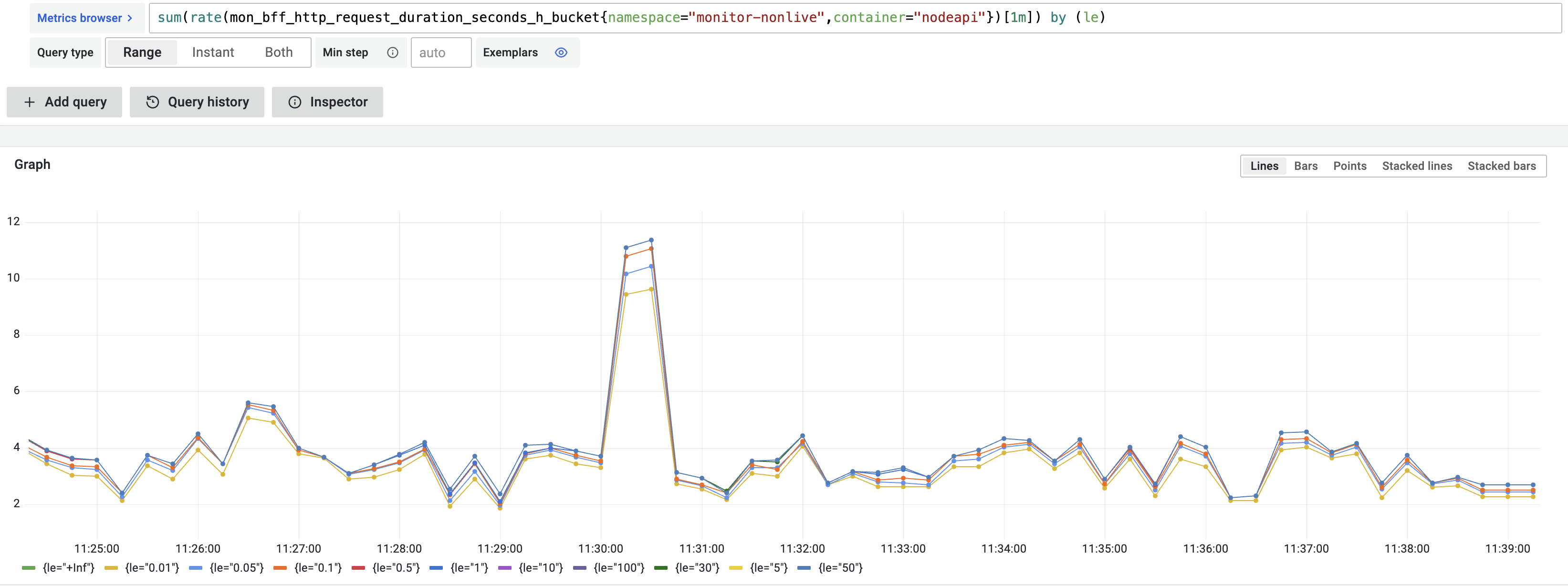
why use rate in the query rate(http_request_duration_seconds_bucket[5m])?
the value of each le of http_request_duration_seconds_bucket is the cumulative count of the requests falling into the bucket, which means the value is increasing over time, but we need the count per second, that’s why rate comes into play. e.g.
before rate:
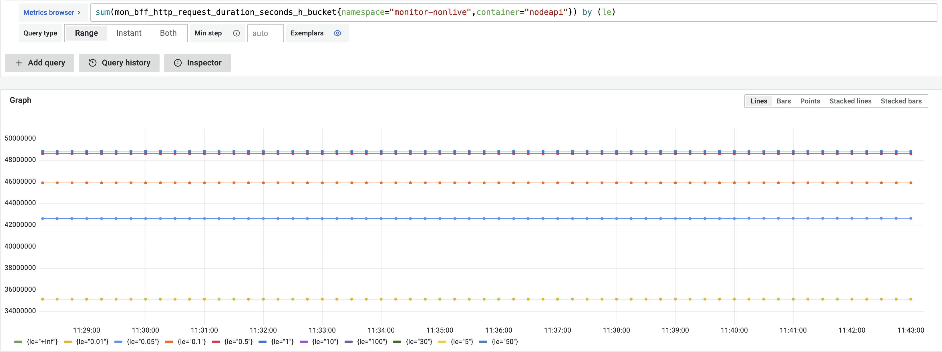
after rate